• Probability and Statistics

Probability and Statistics

⌊x⌋= the greatest integer smaller than x

$$\begin{gathered} \underset{n\to \infty }{\lim }{\left(1+\frac{r}{B}\right)}^A=e^r \\ if \\ \underset{n\to \infty }{\lim }\frac{A^{\prime }}{B^{\prime }}=1 \end{gathered}$$

sequence

index variable

explicit formulas

recurrence relation

arithmetic sequences

geometric sequences

bounded above/ below

(un)bounded

convergent ⇒ bounded

bounded, monotone ⇒ convergent

series

convergent vs divergent series

harmonic sum ${\sum }_{n=1}^{\infty }\frac{1}{n}=\infty$

p series: ${\sum }_{n=1}^{\infty }\frac{1}{n^p}\{\begin{array}{r}convergent,\\ p>1\\ divergent,\\ p\le 1\end{array}$

${\sum }_{n=1}^{\infty }\frac{1}{n^2}=\frac{{\pi }^2}{6}$

${\sum }_{n=k}^{\infty }{a}_n$ convergent ⇒ lim_{n → ∞}a_n = 0

lim_{n → ∞}a_n ≠ 0⇒ ${\sum }_{n=k}^{\infty }{a}_n$ divergent

tests

divergence test

partial sum

geometric: |q| < 1

integral: f, f(n) = a_n, continuous, ultimately decreasing 🡪 same

comparison:

${\lim }_{n\to \infty }\frac{a_n}{b_n}=c\Rightarrow \{\begin{array}{r}same,c\ne 0\\ a_{n}convergent,\\ c=0,\\ b_{n}convergent\\ a_{n}divergent,\\ c=\infty ,\\ b_{n}divergent\end{array}$

scaling with ${\sum }_{n=1}^{\infty }\frac{1}{n^p}(p>1)$ or ${\sum }_{n=1}^{\infty }\frac{1}{n}$

alternating: |a_n + 1| − |a_n| < 0, ∀ n > n₀, lim_{n → ∞}a_n = 0⇒ convergent

absolute convergence: ${\sum }_{}^{}\left|a_n\right|$ convergent

conditional convergence: ${\sum }_{}^{}{a}_n$ convergent, but ${\sum }_{}^{}\left|a_n\right|$ divergent

${\sum }_{}^{}\left|a_n\right|$ convergent $\Rightarrow {\sum }_{}^{}{a}_n$ convergent

ratio: ${\lim }_{n\to \infty }\left|\frac{a_{n+1}}{a_n}\right|\{\begin{array}{r}<1\Rightarrow {\sum }_{}^{}{a}_{n}absolutely\\ convergent\\ >1\Rightarrow {\sum }_{}^{}{a}_{n}divergent\end{array}$

root: ${\lim }_{n\to \infty }\sqrt[n]{|a_n|}\{\begin{array}{r}>1\Rightarrow divergent\\ <1\Rightarrow convergent\end{array}$

uniform convergence:

f_n(x) converge to f(x): f_n(x) → f(x) as n → ∞

∃N(ε) independent to x, ∀n > N, |f_n(x) − f(x)| < ε⇔ uniform convergence: f_n ⇉ f

dominated convergence: f_i(x) → f(x) as x → ∞, ∃g, ∀x, i, f_i(x) < g(x) ⇒ lim_{i → ∞}∫_a^bf_i(x)d**x = ∫_a^bf(x)d**x

power series: ${\sum }_{n=0}^{\infty }{c}_n(x-a{)}^n$

center a, coefficient c_n

 ⇒ x = a⇔ convergent

or ∀x ∈ ℝ, convergent

or ∃R > 0, |x − a| < R⇒ convergent, |x − a| > R⇒ divergent

method: $\rho ={\lim }_{n\to \infty }\left|\frac{c_{n+1}}{c_n}\right|$, radius of convergence $R=\frac{1}{\rho }$

|x − a| < R⇒ absolutely convergent, |x − a| > R⇒ divergent from ratio test

Bessel function of the first kind: $J_0={\sum }_{n=0}^{\infty }\frac{(-1{)}^n{x}^{2n}}{2^{2n}(n!{)}^2}$

basic formula: $$\begin{gathered} \frac{1}{1-x}={\sum }_{n=0}^{\infty }{x}^n \\ for \\ |x|<1 \end{gathered}$$

plug out terms, create (x − a), see something as 1 − x, do it, range

Taylor and Maclaurin Series: $f(x)={\sum }_{n=0}^{\infty }\frac{f^{(n)}(a)}{n!}(x-a{)}^n$

$$\begin{gathered} \frac{1}{1-x}={\sum }_{n=0}^{\infty }{x}^n \\ for \\ |x|<1 \end{gathered}$$

$\ln (1+x)={\sum }_{n=0}^{\infty }(-1{)}^n\frac{x^{n+1}}{n+1}$ for |x| < 1

$-\ln (1-x)={\sum }_{n=1}^{\infty }\frac{x^n}{n}$

$e^x={\sum }_{n=0}^{\infty }\frac{x^n}{n!}$

$\sin x={\sum }_{n=0}^{\infty }(-1{)}^n\frac{x^{2n+1}}{(2n+1)!}$

$\cos x={\sum }_{n=0}^{\infty }(-1{)}^n\frac{x^{2n}}{(2n)!}$

${\tan }^{-1}x={\sum }_{n=0}^{\infty }(-1{)}^n\frac{x^{2n+1}}{2n+1}$ for |x| < 1

$(1+x{)}^k={\sum }_{n=0}^{\infty }\left(\begin{array}{r}k\\ n\end{array}\right)x^n$

$(x+y{)}^k={\sum }_{n=0}^{\infty }\left(\begin{array}{r}k\\ n\end{array}\right)x^n{y}^{k-n}={\sum }_{n=0}^k\left(\begin{array}{r}k\\ n\end{array}\right)x^n{y}^{k-n}$

differentiation and integration: $f^{{}^{\prime }}(x)={\sum }_{n=1}^{\infty }\frac{f^{(n)}(a)}{n!}{\left((x-a{)}^n\right)}^{{}^{\prime }}={\sum }_{n=1}^{\infty }\frac{f^{(n)}(a)}{n!}{n(x-a)}^{n-1}$, ${\int }_{}^{}f(x)dx={\sum }_{n=0}^{\infty }\frac{f^{(n)}(a)}{n!}{\int }_{}^{}(x-a{)}^{n}dx={\sum }_{n=0}^{\infty }\frac{f^{(n)}(a)}{n!}\frac{(x-a{)}^{n+1}}{n+1}+C$

may lose boundary of convergence

Cauchy product: $f(x)g(x)={\sum }_{n=0}^{\infty }{a}_n{x}^n{\sum }_{n=0}^{\infty }{b}_n{x}^n={\sum }_{n=0}^{\infty }{c}_n{x}^n$, $c_n={\sum }_{k=0}^{\infty }{a}_k{b}_{n-k}$

$\left(\begin{array}{r}k\\ n\end{array}\right)=\frac{k!}{n!(k-n)!}=\frac{k(k-1)\dots (k-n+1)}{n!}$

probability

sample space S: nonempty set

collection of events: subset of S: P(S)

probability measure P(A) ∈ [0, 1], P(⌀) = 0, P(S) = 1

$P\left({\bigcup }_{i=1}^n{A}_i\right)={\sum }_{i=1}^{n}P\left(A_i\right)$ if A_i… are mutually disjoint

symmetric difference: AΔB = (A ∖ B) ∪ (B ∖ A)

complement: A^c :  = S ∖ A

disjoint: A ∩ B = ⌀ ⇔ A ⊆ B^c ⇒ A ∖ B = A ∩ B^c

De Morgan Laws: (A ∪ B)^c = A^c ∩ B^c, (A ∩ B)^c = A^c ∪ B^c

A = B ⇔ A ⊆ B, B ⊆ A

cardinality: |A|= # of elements in A

inclusion-exclusion principle: |A ∪ B| = |A| + |B| − |A ∩ B|, |A ∪ B ∪ C| = |A| + |B| + |C| − |A ∩ B| − |A ∩ C| − |B ∩ C| + |A ∩ B ∩ C|

partition of the sample: B_i, disjoint, S = B₁ ∪ B₂ ∪ …

P(A) = P(A ∩ B₁) + P(A ∩ B₂) + …

P(A ∖ B) = P(A ∩ B^c) = P(A) − P(B)

not necessarily disjoint: P(A₁ ∩ A₂ ∩ …) ≤ P(A₁) + P(A₂) + …

independent: P(A ∩ B) = P(A)P(B) for two events, and P(A₁ ∩ … ∩ A_i) = P(A₁)…P(A_i) for more events

uniform probability: $P(A)=\frac{|A|}{|S|}$

continuous uniform distribution: $P\left([x,y]\right)=\frac{y-x}{b-a}$, [x, y] ⊂ [a, b]

combinatorics: length k, n symbols  ⇒ n^k

ordered subset $\Rightarrow {\frac{n!}{(n-k)!}=n}^{\underline{k}}$

binomial: $$\begin{gathered} \left(\begin{array}{r}n\\ k\end{array}\right)=\frac{n!}{k!(n-k)!},or \\ 0 \\ if \\ k<0 \\ or \\ k>n \end{gathered}$$

$\left(\begin{array}{r}n\\ k\end{array}\right)=\left(\begin{array}{r}n-1\\ k\end{array}\right)+\left(\begin{array}{r}n-1\\ k-1\end{array}\right)$

$\left(\begin{array}{r}2n\\ n\end{array}\right)={\sum }_{k=0}^n{\left(\begin{array}{r}n\\ k\end{array}\right)}^2$

generating function: $f(x)={\sum }_{n=0}^{\infty }{a}_n{x}^n$

exponential generating function: $f(x)={\sum }_{n=0}^{\infty }{a}_n\frac{x^n}{n}$

Bayes’ theorem: $P\left(B|A\right)=\frac{P(B\cap A)}{P(A)}=\frac{P(B)}{P(A)}P\left(A|B\right)$

random variable X(bla) = 2

discrete: ${\sum }_{x\in \mathbb{R}}^{}P(X=x)=1$

PDF probability mass/ density function: p_X(x) = P(X = x)

$P(X=x)={\sum }_i^{}P\left(A_i\right)P(X=x|A_i)$

law of total probability: $P(A)={\sum }_{x\in \mathbb{R}}^{}P(X=x)P\left(A|X=x\right)$

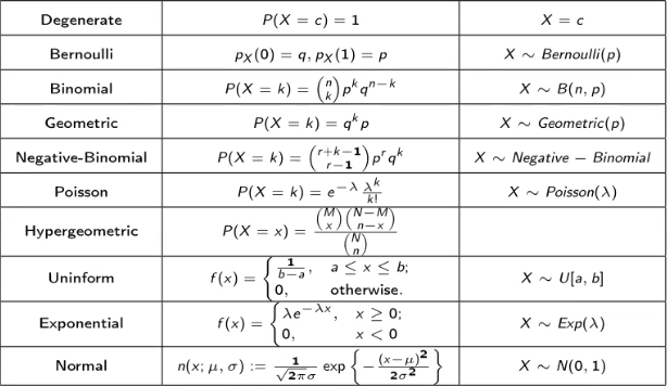
Bernoulli: p_X(0) = q, p_X(1) = p

Binomial: $p_X(k)=\left(\begin{array}{r}n\\ k\end{array}\right)p^k{q}^{n-k}$

r_X(t) = (t**p + q)ⁿ

geometric: p_X(k) = p**q^k

$E(X)=\frac{q}{p},var(X)=\frac{q}{p^2}$

negative-binomial: $p_X(k)=\left(\begin{array}{r}r+k-1\\ k\end{array}\right)p^r{q}^k=(-1{)}^k\left(\begin{array}{r}-r\\ k\end{array}\right)p^r{q}^k$

Poisson: $p_X(k)=e^{-\lambda }\frac{{\lambda }^k}{k!}$

E(X) = var(X) = λ

hypergeometric: $p_X(k)=\frac{\left(\begin{array}{r}M\\ k\end{array}\right)\left(\begin{array}{r}N-M\\ n-k\end{array}\right)}{\left(\begin{array}{r}n\\ N\end{array}\right)}$

continuous distribution: p_X(k) = 0 ∀ x ∈ ℝ,∫_−∞^∞f(x)d**x = 1

uniform: $f(x)=\{\begin{array}{r}\frac{1}{b-a},a\le x\le b\\ 0\end{array}$

$var(X)=\frac{(b-a{)}^2}{12}$

exponential: $f(x)=\{\begin{array}{r}\lambda e^{-\lambda x},0\le x\\ 0,x<0\end{array}$

P(x ≥ t) = e^−λ**t

$E(X)=\frac{1}{\lambda },var(X)=\frac{1}{{\lambda }^2}$

$$\begin{gathered} r_X(t)=\frac{\lambda }{\lambda -\ln t} \\ if \\ \lambda -\ln t>0 \end{gathered}$$

normal: $f(x)=n\left(x;\mu ,{\sigma }^2\right):=\frac{1}{\sqrt{2\pi }\sigma }{e}^{-\frac{(x-\mu {)}^2}{2{\sigma }^2}}$

$\Phi (x)=\frac{1}{\sqrt{2\pi }}{\int }_{-\infty }^x{e}^{-\frac{t^2}{2}}dt$

gamma: $f(x)=\{\begin{array}{r}\frac{{\lambda }^{\alpha }{x}^{\alpha -1}}{\Gamma (\alpha )}{e}^{-\lambda x},x\ge 0\\ 0,x<0\end{array}$

$\Gamma (x)={\int }_0^{\infty }{t}^{x-1}{e}^{-t}dt=\{\begin{array}{r}(x-1)!,x\in N\ast \\ \sqrt{\pi },x=\frac{1}{2}\end{array}$

Γ(x + 1) = x**Γ(x)

chi-squared: Χ²(n) is the distribution of Z = X₁² + … + X_n² with X_i ∼ N(0, 1)

$Z\sim \Gamma \left(\frac{n}{2},\frac{1}{2}\right)$

E(Z) = n

$f_Z(z)=\frac{1}{\sqrt{2\pi z}}{e}^{-\frac{z}{2}}$ for z ≥ 0 if n = 1

t (or student): t(n) is the distribution of $Z=\frac{X}{\sqrt{\frac{X_1^2+\dots +X_n^2}{n}}}$ with X_i ∼ N(0, 1)

$T=\frac{\overline{X}-\mu }{\frac{{\overline{S}}_n}{\sqrt{n}}}\sim t(n-1)$

CDF cumulative distribution fun $F_X(x)=P(X\le x)=\{\begin{array}{r}{\sum }_{y_i\le x}^{}{f}_X\left(y_i\right),discrete\\ {\int }_{-\infty }^x{f}_X(t)dt,continuous\end{array}$

joint distributions Y = h(X)

if X discrete, then $$\begin{gathered} P_Y(y)={\sum }_{x\in h^{-1} \\ y \\ }^{}{P}_X(x) \end{gathered}$$

if X continuous, h(x) monotone where f_X(x) > 0, then $f_Y(y)=\frac{f_X\left(h^{-1}(y)\right)}{{|h}^{{}^{\prime }}\left(h^{-1}(y)\right)|}$

marginal distribution: F_X(x) = lim_{y → ∞}F_X, Y(x, y)

joint probability fun

marginal PDF: $p_X(x)={\sum }_y^{}{p}_{X,Y}(x,y)$ table

joint density fun: f(x, y), ∫_−∞^∞∫_−∞^∞f(x, y)dxd**y = 1

marginal PDF f_X(x) = ∫_−∞^∞f_X, Y(x, y)d**y

independent $P\left(A|B\right)=\frac{P(A\cap B)}{P(B)}$

$p_{Y|X}\left(y|x\right)=\frac{p_{X,Y}(x,y)}{{\sum }_z^{}{p}_{X,Y}(x,z)}=\frac{p_{X,Y}(x,y)}{p_X(x)}$ or f

continuous: $P(a\le Y\le b,X=x)={\int }_a^b\frac{f_{X,Y}(x,y)dy}{f_X(x)}$

law of total prob: P((X, Y) ∈ B) = ∬_Bf_X(x)f_Y|X(y|x)dxd**y

independent random variables: ∀B₁, B₂, P(X ∈ B₁, Y ∈ B₂) = P(X ∈ B₁)P(Y ∈ B₂)

expectation: E(X**Y) = E(X)E(Y) if X, Y independent

variance: var(X) = E((X − μ_x)²) = E(X²) − E²(X), var(X + Y) = var(X) + var(Y) + 2cov(X, Y)

covariance: cov(X, Y) = E((X − μ_X)(Y − μ_Y)) = E(X**Y) − E(X)E(Y)

cov(a**X + b**Y, Z) = a cov(X, Z) + b cov(Y, Z)

correlation: $corr(X,Y)=\frac{cov(X,Y)}{Sd(X)Sd(Y)}$

i.i.d. mutually independent and identically distributed

X₁, …, X_n ∼ Bernoulli(p) i. i. d.  ⇒ X₁ + … + X_n ∼ B(n, p)

X₁ ∼ B(n₁, p), X₂ ∼ B(n₂, p) ⇒ X₁ + X₂ ∼ B(n₁ + n₂, p)

X₁ ∼ Poisson(λ₁), X₂ ∼ Poisson(λ₂) ⇒ X₁ + X₂ ∼ Poisson(λ₁ + λ₂)

generating fun: r_X(t) = E(t^X)

r_X + Y(t) = r_X(t)r_Y(t)

kth moment: E(X^k)

kth central moment: E((X − μ_x)^k)

moment-generating fun: $M_X(s)=E\left(e^{Xs}\right)=r_X\left(e^s\right)={\sum }_{n=0}^{\infty }\frac{E\left(X^n\right)}{n!}{s}^n$

M_X^(k)(0) = E(X^k)

M_X + Y(s) = M_X(s)M_Y(s) X, Y independent, work for r_X(t)

uniqueness: if ∃s₀ > 0, M_X(s) < ∞ ∀s ∈ (−s₀, s₀), M_X(s) = M_Y(s), then X, Y have the same distribution also work for r

characteristic fun: c_X(s)= E(e^iXs)

inequalities

Markov’s:$P(X\ge a)\le \frac{E(X)}{a}$ X ≥ 0, a > 0

Chebychev’s: $P\left(\left|X-{\mu }_X\right|\ge a\right)\le \frac{var(X)}{a^2}$ a > 0

Cauchy-Schwarz: $\left|cov(X,Y)\right|\le \sqrt{var(X)var(Y)}$

=, iff $X-{\mu }_X=\frac{cov(X,Y)}{var(Y)}(Y-{\mu }_Y)$ if var(Y) > 0

law of large number

sample sum: S_n = X₁ + … + X_n for {X_i} i. i. d.

sample average: $M_n=\overline{X}=\frac{1}{n}\left(X_1+\dots +X_n\right)=\frac{S_n}{n}$

WLLN weak: lim_{n → ∞}P(|M_n − μ| ≥ ε) = 0 for {X_i} same μ, var ≤ v, v < ∞, ε > 0 not necessarily i. i. d.

$M_n\stackrel{P}{\to }\mu$

SLLN strong: P{lim_{n → ∞}M_n = μ} = 1 for {X_i} i. i. d.

$M_n\stackrel{a.s.}{\to }\mu$x

central limit theorem: lim_{n → ∞}P(Z_n ≤ x) = P(Z ≤ x) for {X_i} i. i. d, Z ∼ N(0, 1), $Z_n=\frac{S_n-n\mu }{\sqrt{n}\sigma }=\sqrt{n}\left(\frac{M_n-\mu }{\sigma }\right)$

$\Phi (x)={\lim }_{n\to \infty }P\left(Z_n\le x\right)={\lim }_{n\to \infty }P\left(S_n\le n\mu +x\sqrt{n}\sigma \right)={\lim }_{n\to \infty }P\left(M_n\le \mu +\frac{x\sigma }{\sqrt{n}}\right)$

$Z_n\stackrel{D}{\to }Z\sim N(0,1)$

convolution: for X, Y independent, Z = X + Y

discrete: $p_Z(z)={\sum }_w^{}{p}_X(z-w)p_Y(w)$

continuous: f_Z(z) = ∫_−∞^∞f_X(z − w)f_Y(w)d**w

different convergence

$X_n\stackrel{P}{\to }Y$: {X_n} converges in probability to Y, if lim_{n → ∞}P(|X_n − Y| ≥ ε) = 0

$X_n\stackrel{a.s.}{\to }Y$: {X_n} converges with probability 1 (almost surely) to Y, if lim_{n → ∞}P(X_n = Y) = 1

$X_n\stackrel{D}{\to }Y$: {X_n} converges in distribution to Y, if lim_{n → ∞}P(X_n ≤ x) = P(Y ≤ x) ∀ x ∈ {x|P(Y = x) = 0}

$X_n\stackrel{a.s.}{\to }Y\Rightarrow X_n\stackrel{D}{\to }Y\Rightarrow X_n\stackrel{P}{\to }Y$

sample

sample variance: $\overline{S_n^2}=\frac{1}{n-1}{\sum }_{j=1}^n{\left(X_j-\overline{X}\right)}^2$

kth sample moment: $\overline{x^k}$

point estimation

the method of moments:  ${\hat{\mu }}_n=\overline{X},{\hat{\sigma }}^2=\overline{X^2}-{\overline{X}}^2$

MLE maximum likelihood estimation: make L big as possible

maximum likelihood fun: L(θ; x₁, …, x_n) = p(X₁ = x₁, …X_n = x_n|θ) or f

x₁, …, x_n independent: $L\left(\theta ;x_1,\dots ,x_n\right)={\prod }_{j=1}^{n}p\left(X_j=x_j|\theta \right)$

good point estimator

unbiased: E(θ̂_n) = θ

consistent: ${\hat{\theta }}_n\stackrel{P}{\to }\theta$

mean squared error E((θ̂_n − θ)²) is small

confidence interval: P(θ̂_n⁻ ≤ θ ≤ θ̂_n⁺) ≥ 1 − α

 ⇐ P(a ≤ g(θ) ≤ b) ≥ 1 − α

N, t: let −b = a,

Χ²: let $a=X_{\frac{\alpha }{2}}^2(n),b=X_{1-\frac{\alpha }{2}}^2(n)$

deal with X_i ∼ N(μ, σ²)

 ${\overline{S}}^2=\frac{1}{n-1}{\sum }_{i=1}^n{\left(X_i-\overline{X}\right)}^2$

$\sigma ={\sigma }_0\Rightarrow \frac{\overline{X}-\mu }{{\sigma }_0/\sqrt{n}}\sim N(0,1)\Rightarrow \mu$

$\frac{\overline{X}-\mu }{{\overline{S}}_n/\sqrt{n}}\sim t(n-1)\Rightarrow \mu$

μ = μ₀: $\frac{1}{{\sigma }^2}{\sum }_{i=1}^n{\left(X_i-{\mu }_0\right)}^2\sim X^2(n)\Rightarrow \sigma$

$\frac{(n-1){\overline{S}}^2}{{\sigma }^2}\sim X^2(n-1)\Rightarrow \sigma$

hypothesis testing

null hypothesis H₀

type I/ II error: H₀ true/ false

level of significance α: probability for type I error

power of the test 1 − β, β: probability for type II error

p-value: probability that H₀ is true

reject if p-value  < α

for {X_i ∼ N(μ, σ₀²)} i.i.d., use $\frac{\overline{X}-{\mu }_0}{{\sigma }_0/\sqrt{n}}\sim N(0,1)$

for two samples, $T=\frac{\left({\overline{X}}_1-{\mu }_1\right)-({\overline{X}}_2-{\mu }_2)}{\sqrt{\frac{S_1^2}{n_1}+\frac{S_2^2}{n_2}}}\sim t(df),df=\frac{{\left(\frac{S_1^2}{n_1}+\frac{S_2^2}{n_2}\right)}^2}{\frac{1}{n_1-1}{\left(\frac{S_1^2}{n_1}\right)}^2+\frac{1}{n_2-1}{\left(\frac{S_2^2}{n_2}\right)}^2}$

linear regression

linear least squares $\{\begin{array}{r}m=\frac{{\sum }_{j=1}^n\left(x_j-\overline{x}\right)\left(y_j-\overline{y}\right)}{{\sum }_{j=1}^n(x_j-\overline{x})}\\ b=\overline{y}-m\overline{x}\end{array}$

correlation coefficient: $r=corr(X,Y)=\frac{n{\sum }_{j=1}^n\left(x_j{y}_j\right)-{\sum }_{j=1}^n{x}_j{\sum }_{j=1}^n{y}_j}{\sqrt{\left[{\sum }_{j=1}^n{x}_j^2-{\left({\sum }_{j=1}^n{x}_j\right)}^2\right]\left[{\sum }_{j=1}^n{y}_j^2-{\left({\sum }_{j=1}^n{y}_j\right)}^2\right]}}$

standard statistical model: Y_j = β₀ + β₁x_j + e_j, j = 1, 2, …, n

E(e_j) = 0, var(e_j) = σ²

intercept β₀, slope β₁, residual e_j

estimators $\{\begin{array}{r}{\hat{\beta }}_1=\frac{1}{l_{XX}}{\sum }_{j=1}^n\left(x_j-\overline{x}\right)\left(y_j-\overline{y}\right)=\frac{1}{l_{XX}}\left({\sum }_{j=1}^n{x}_j{y}_j-n\overline{x}\overline{y}\right)\\ {\hat{\beta }}_0=\frac{{\sum }_{j=1}^n{x}_j^2{\sum }_{j=1}^n{y}_j-{\sum }_{j=1}^n{x}_j{\sum }_{j=1}^n{x}_j{y}_j}{n{\sum }_{j=1}^n{x}_j^2-{\left({\sum }_{j=1}^n{x}_j\right)}^2}\end{array}$

$$l_{XX}=\sum _{j=1}^n{\left(x_j-\overline{x}\right)}^2=\sum _{j=1}^n{x}_j^2-n{\overline{x}}^2$$

E(β̂₀) = β₀, E(β̂₁) = β₁

$var\left({\hat{\beta }}_0\right)=\left(\frac{1}{n}+\frac{{\overline{x}}^2}{l_{XX}}\right){\sigma }^2,var\left({\hat{\beta }}_1\right)=\frac{{\sigma }^2}{l_{XX}},cov\left({\hat{\beta }}_0,{\hat{\beta }}_1\right)=-\frac{\overline{x}}{l_{XX}}{\sigma }^2$

if e_j ∼ N(0, σ²) i.i.d., then β̂₀, β̂₁ normal dist

sum of squared errors SSE: $S_e^2={\sum }_{j=1}^n{\left(Y_j-{\hat{\beta }}_0-{\hat{\beta }}_1{x}_j\right)}^2$

${\hat{\sigma }}^2=\frac{S_e^2}{n-2}$

$E\left({\hat{\sigma }}^2\right)={\sigma }^2,\frac{S_e^2}{{\sigma }^2}\sim X^2(n-2),{\hat{\sigma }}^2$ independent of β̂₀, β̂₁

$$\begin{gathered} \sigma \\ known\frac{{\hat{\beta }}_1-{\beta }_1}{\sigma /\sqrt{l_{XX}}}\sim N(0,1)\Rightarrow {\hat{\beta }}_1 \end{gathered}$$

$$\frac{{\hat{\beta }}_1-{\beta }_1}{\hat{\sigma }/\sqrt{l_{XX}}}\sim t(n-2)\Rightarrow {\hat{\beta }}_1$$

$$\begin{gathered} \sigma \\ known\frac{{\hat{\beta }}_0-{\beta }_0}{\sigma /\sqrt{\frac{1}{n}+\frac{{\overline{x}}^2}{l_{XX}}}}\sim N(0,1)\Rightarrow {\hat{\beta }}_0 \end{gathered}$$

$$\frac{{\hat{\beta }}_0-{\beta }_0}{\hat{\sigma }/\sqrt{\frac{1}{n}+\frac{{\overline{x}}^2}{l_{XX}}}}\sim t(n-2)\Rightarrow {\hat{\beta }}_0$$

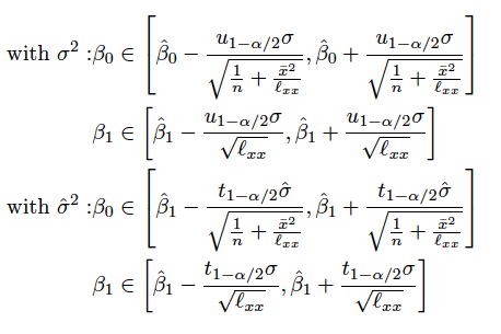
1 − α confidence interval for β̂₀, β̂₁

1 − α confidence interval for σ²

$$\left[\frac{(n-2){\hat{\sigma }}^2}{X_{\frac{\alpha }{2}}^2(n-2)},\frac{(n-2){\hat{\sigma }}^2}{X_{1-\frac{\alpha }{2}}^2(n-2)}\right]$$

${\hat{y}}_0\sim N\left({\beta }_0+{\beta }_1{x}_0,\left(\frac{1}{n}+\frac{{\left(x_0-\overline{x}\right)}^2}{l_{XX}}\right){\sigma }^2\right)$

1 − α confidence interval for y₀ = E(ŷ₀): $\left[y_0-t_{1-\frac{\alpha }{2}}(n-2)\hat{\sigma }\sqrt{\frac{1}{n}+\frac{{\left(x_0-\overline{x}\right)}^2}{l_{XX}}},y_0+t_{1-\frac{\alpha }{2}}(n-2)\hat{\sigma }\sqrt{\frac{1}{n}+\frac{{\left(x_0-\overline{x}\right)}^2}{l_{XX}}}\right]$